This blog post outlines a recent paper which I worked on with my fantastic collaborators Joel Dyer and Arnau Quera-Bofarull. This work was published at AAMAS 2024 - check out the full paper here!

Synthetic Populations and ABMs

Designing an agent-based model (ABM) invetiably invovles generating a population of agents. Typically, modellers rely on datasets describing the underlying real-world population they are seeking to emulate. Armed with this data, the modeller can use their favourite algorithm to generate a population of agents with realistic statistics. For instance, many practitioners use iterative proportional fitting (which economists often call raking) to generate a synthetic population that has the correct marginal statistics using cross-table data.

So, what is the problem with this approach? It seems completely reasonable, but there are some issues. Firstly, the modeller might not have access to real-world data. This could be due to privacy concerns, or simply because the required data wasn’t collected in the first place. In addition, the agent-based model is never used to inform population design. Say you are an epidemiologist who has built an epidemic simulator for the UK. If you run your simulator and every individual gets infected within a single day, you may suspect that your synthetic population is not very representative.

In this work, we provide an altenative approach for generating synthetic populations which directly leverages the ABM. In what follows, we will think of an ABM as a stochastic simulator \(p\), which takes a set of structural parameters \(\omega\) as well as an population of agents \(\mathcal{A}_{N}\) and produces an output state \(x \in \mathcal{X}\).

\[x \sim p(\cdot \mid \omega, \mathcal{A}_{N})\]

Stuctural parameters represent global factors in the ABM which are not specific to any particular agent. Staying with our epidemic example, structural parameters may include vaccine efficacy or the infectiousness of the virus.

Generating Simulation Outputs from an ABM

For now, let us assume we have access to a domain expert, who has perfect knowledge of the structural parameters and the true underlying population. In this case, the process of simulating from our ABM may look as follows:

graph LR
    expert("Domain Expert")
    struct("Structural Parameters")
    pop("Agent Population")
    sim("ABM")
    state("Output State")

    expert --> struct & pop
    struct & pop --> sim
    sim --> state 

That is, we query the domain expert for the structural paramaters \(\omega\) and population \(\mathcal{A}_{N}\) then forward-simulate the ABM \(p\) to get an output state \(x \in \mathcal{X}\). Of course, a domain expert rarely has perfect information. As already discussed, the domain expert may have insufficient data to estimate population structure. Likewise, the domain expert may have imperfect knowledge about the structural parameters. In the worst-case the modeller may not even have access to a domain expert at all!

In our work, we aim to resolve these issues by replacing the domain expert in the diagram above with a proposal distribution \(q\) which aims to generate good sturctural parameters and populations. Instead of generating both the population and structural parameters jointly from the proposal distribution in one step, we generate structural parameters and population parameters \(\theta\) from the proposal distribution. The population parameters are used to parameterise an attribute distribution \(f\) from which the agent population is finally generated.

\[\mathcal{A}_{N} \sim f(\cdot \mid \theta)\]

Once we have the agent population and the structural parameters, we can proceed as before and forward-simulate the ABM to get an output state \(x \in \mathcal{X}\). Our approach is summarised by the following diagram:

graph TD
    prop("Proposal distribution")
    param("Population parameters")
    attr("Attribute distribution")
    struct("Structural Parameters")
    pop("Agent Population")
    sim("ABM")
    state("Output State")

    prop --> param & struct
    param --> attr
    attr --> pop
    struct & pop --> sim
    sim --> state

Of course, in order for this approach to work we need to pick a good proposal distribution. In learning the proposal distirbution, we suffer from similar issues to a domain expert that lacks knowledge or data. However, typically a modeller knows what kind of outputs they are interested in. For example, an epidemiologist may be trying to fit their ABM to a real-world time series \((y_{t})^{T}_{t=1}\), or they may be interested in searching for populations where the risk of contagion (number of infected citizens) is high. Our key idea is that the modeller’s preferences over state outputs can be used in conjunction with the ABM to learn a good proposal distribution.

Learning a Proposal Distirbution

In order to do this, we assume that the modeller/domain expert has provided us with a loss function \(\ell: \mathcal{X} \to \mathbb{R}_{+}\) describing their preferences over ABM outputs. For example, an epidemiologist trying to fit to a real-world time series of infections \((y_{t})^{T}_{t=1}\) may propose the following loss function:

\[\ell(x) = \frac{1}{T}\sum^{T}_{t=1}(y_{t} - x_{t})^{2}\]

where we have assumed the output of the simulator is a time-series of infections \(x = (x_{t})_{t=1}^{T}\). Alternatively, let’s assume the epidemiologist is interested in any outcome where more than \(\tau\) individuals are infected. In this case, the epdemiologist may choose the following loss function:

\[\ell(x) = \mathbb{I}(\cdot \leq \tau)(x)\]

where we have assumed the output \(x\) of the ABM describes the total number of infections over the simulation run. Here \(\mathbb{I}(\cdot \geq \tau)\) denotes the indicator function that reuturns \(1\) when \(x\) is less than \(\tau\) and \(0\) otherwise.

Given the loss function \(\ell\), we propose many algorithms for learning a good proposal distribution \(q\) by repeatedly sampling simulation runs from the ABM. Note that our approaches require no external data once the loss function has been defined! Next, I will walkthrough my favourite method for learning \(q\). You can check out other methodologies in the paper!

Learning a Proposal Distribution through Variational Optimisation

One way to learn a suitable proposal distribution is to take a variational approach. That is, we may consider a parameterised family of proposal distributions:

\[\mathcal{Q} = \{q(\cdot \mid \phi) \mid \phi \in \Phi\}.\]

In our experiments, we take \(\mathcal{Q}\) to be a normalizing flow. Then, to select an ideal proposal distribution \(q^{\star}\) from \(\mathcal{Q}\), we solve the following variational optimisation problem:

\[q^{\star} = \arg\min_{\phi \in \Phi} \left\{ \mathbb{E}_{\omega, \theta \sim q(\omega, \theta)} \left[\mathcal{L}(\omega, \theta)\right] - \gamma \mathbb{H}(q(\cdot \mid \phi)) \right\}.\]

Here, \(\mathcal{L}\) denotes a lifted loss over the structural and population parameters \((\omega, \theta)\) constructed using the domain expert supplied loss \(\ell\):

\[\mathcal{L}(\omega, \theta) = \mathbb{E}_{x \sim p(x \mid \omega, \theta)} \left[ \ell(x) \right].\]

Roughly speaking, \(\mathcal{L}(\omega, \theta)\) captures the average loss experienced by the domain expert when \(\omega\) and \(\theta\) are used to forward-simulate the ABM using the approach outlined in the previous diagram. As a result, the first term in the objective above captures the average loss experienced by the domain expert when structural parameters and population parameters are sampled from the proposal distirbution \(q\).

Meanwhile \(\mathbb{H}\) denotes the entropy function. Thus the second term penalises the proposal distribution for accumulating too much probability mass on a small subset of structural and population parameter values. The trade-off between both terms is controlled by the scalar parameter \(\gamma > 0\) which the modeller is free to choose. Note that a large \(\gamma\) will encourage greater diversity, whilst setting \(\gamma = 0\) causes \(q^{\star}\) to collapse to a degenerate distribution whose mass is concentrated on the pairs \((\omega, \theta)\) that minimise \(\mathcal{L}\).

As mentioned before, we use normalising flows in our experiments to define the variational family \(\mathcal{Q}\). As a result, we can readily solve the variational problem above by performing stochastic gradient descent on the paramaters \(\phi\), which correspond to network weights within the normalising flow.

A Simple Example

To finish, let’s run through a simple example of our approach. We will consider Axtell’s model of firms. This model studies the evolution of financial firms over time. The model consists of a set of agents, who each belong to a particular firm at each time step. Each agent \(n\) works with some effort level \(e^{t}_{n} \in [0, 1]\) at time \(t\) and periodically reeavluates their situation at an agent-specific rate \(\rho_{n}\). In addition, each agent maintains a parameter \(\nu_{n} \in [0, 1]\) describing their preference for leisure vs income. When reevaluating, agents decide between

• adjusting their effort level
• moving to an existing firm
• or starting a new firm.

You can find full details about the model in our paper. Now assume that we are a modeller interested in the following question:

Can an initially hardworking population become lazy over time?

To answer this question we first need to construct a suitable loss function. In this case, we can choose a simple loss function that measures the difference between the average effort of agents at the beginning and end of the time horizon:

\[\ell(x) = \frac{1}{N}\sum^{N}_{n=1}\left(e^{1}_{n} - e^{0}_{n}\right),\]

where \(x = (e^{t})_{t=1}^{T}\) is a time series of vectors describing the effort-level of each agent on each time step. We also need to define a parameterised family of attribute distributions. For the sake of simplicity and interpretability, we will assume that each agent’s features are generated independently and identically from a product of beta and gamma distributions:

\[f(e^{0}_{n}, \nu_{n}, \rho_{n} \mid \theta) = \text{Beta}(e_n^0 \mid \varepsilon_{a}, \varepsilon_b) \cdot \text{Beta}(\nu_n \mid g_a, g_b) \cdot \text{Gamma}(\rho_n \mid \varrho_a, \varrho_b)\]

where \(\theta = (\varepsilon_{a}, \varepsilon_b, g_a, g_b, \varrho_a, \varrho_b)\). There are no structural parameters in this model, so we don’t need to worry about them.

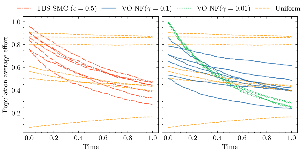
We are now ready to learn a proposal distribution. The plot below shows the average effort of agents over time from simulation runs generated by different proposal distributions. In particular, the right-hand plot shows simulation runs generated by proposal distributions trained with our variational approach for different values of \(\gamma\). When comparing these runs to those generated from a uniform proposal distribution we see a marked difference. Proposal distributions trained via our variational approach consistently produce populations with decaying effort over time.

Since our attribute distribution is simple, we can look at our proposal distributions and see what is causing this decay in effort.

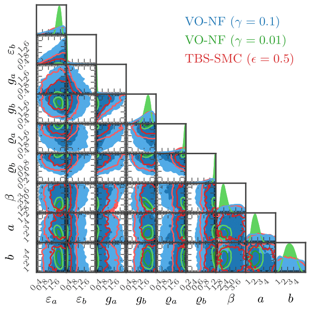
The blue and green plots correspond to proposal distributions we found using variational optimisation. We can make several observations immediately:

• Agents need to begin with high effort levels. This is evidenced by the proposal distributions assigning higher density to larger/lower values of \(\varepsilon_{a}\) and \(\varepsilon_{b}\) respectively.
• Agents need to reeavluate their position on a relatively frequent basis. This is manifested by relatively high/low densities assigned to \(g_{a}\) and \(g_{b}\) respectively, which translates to a left-skewed distribution over \(\nu_{n}\).
• Agents need a strong preference for leisure over income. This is manifested by high density assigned to both \(\varrho_{a}\) and \(\varrho_{b}\), which increases the mass assigned by the gamma distribution to higher values of \(\rho_{n}\).

Check out the full paper for more examples!

Code

If you want to apply our framework in your own research I highly recommend checking out SynthPop, which is a Python package we developed for precisely this reason!